CliffordNet: All You Need is Geometric Algebra




“The two systems [Hamilton’s and Grassmann’s] are not only consistent with one another, but they are actually parts of a larger whole.”
— William Kingdon Clifford, 1878
Official implementation of the paper "CliffordNet: All You Need is Geometric Algebra".
We introduce Clifford Algebra Network (CAN), a novel vision backbone that challenges the necessity of Feed-Forward Networks (FFNs) in deep learning. By operationalizing the full Clifford Geometric Product ($uv = u \cdot v + u \wedge v$), we unify feature coherence and structural variation into a single, algebraically complete interaction layer.
Our "No-FFN" variant demonstrates that this geometric interaction is so expressive that heavy MLPs become redundant, establishing a new Pareto frontier for efficient visual representation learning.
🚀 News & Updates
- [2026-03-01] ⚡ A backbone with a pyramid structure has been added.
- [2026-02-17] 🔥 Released the code for preliminary experiments on CIFAR-100.
- [2026-01-20] 🏆 New SOTA:
- Nano (1.4M) reaches 77.82%, outperforming ResNet-18 (11M).
- Lite (2.6M) reaches 79.05% without FFN, rivaling ResNet-50.
- 32-Layer Deep Model achieves 81.42% with only 4.8M parameters.
- [2026-01-12] ⚡ Performance Preview: We have successfully implemented a custom Fused Triton Kernel for the Clifford Interaction layer. Preliminary benchmarks on RTX 4090 show a 10x kernel speedup and ~2x end-to-end training speedup. Code coming soon!
- [2026-01-01] 🏆 SOTA on CIFAR-100: Our Nano model (1.4M) matches ResNet-18 (11M), and our No-FFN model outperforms MobileNetV2 by >6%.
🏆 Main Results (CIFAR-100)
We compare CliffordNet against established efficient backbones under a rigorous "Modern Training Recipe" (200 Epochs, AdamW, AutoAugment, DropPath).
Efficiency & Performance
| Model Variant | Params | MLP Ratio | Context Mode | Top-1 Acc | vs. Baseline |
|---|---|---|---|---|---|
| Baselines | |||||
| MobileNetV2 | 2.3M | - | - | 70.90% | - |
| ShuffleNetV2 1.5x | 2.6M | - | - | 75.95% | - |
| ResNet-18 | 11.2M | - | - | 76.75% | - |
| ResNet-50 | 23.7M | - | - | 79.14% | - |
| CliffordNet (Ours) | |||||
| CAN-Nano | 1.4M | 0.0 | Diff ($\Delta H$) | 77.82% | > ResNet-18 |
| CAN-Lite | 2.6M | 0.0 | Diff ($\Delta H$) | 79.05% | ~ ResNet-50 |
| CAN-32 | 4.8M | 0.0 | Diff ($\Delta H$) | 81.42% | SOTA |
| CAN-64 (Deep) | 8.6M | 0.0 | Diff ($\Delta H$) | 82.46% | SOTA |
| CAN-96 (Deep) | 12.8M | 0.0 | Diff ($\Delta H$) | 83.47% | SOTA |
Key Insight: Our Nano variant (1.4M) outperforms the heavy-weight ResNet-18 (11.2M) by +1.07% while using $8\times$ fewer parameters. The Lite variant (No-FFN) effectively matches ResNet-50 with $9\times$ fewer parameters.
🏗️ Architecture & Theory
The evolution of features in CliffordNet is governed by a Geometric Diffusion-Reaction Equation. We introduce a unified superposition principle that integrates local differential context and global mean fields:
$$ \frac{\partial H}{\partial t} = \mathcal{P}{loc}\Big( H (\mathcal{C}{loc}) \Big) + \beta \cdot \mathcal{P}{glo}\Big( H (\mathcal{C}{glo}) \Big) $$
Where $\mathcal{C}{loc} \approx \Delta H$ (Local Laplacian) and $\mathcal{C}{glo} = \text{GlobalAvg}(H)$. The interaction term is expanded via the Clifford Geometric Product, unifying scalar and bivector components:
$$ \mathcal{P}\Big( H(\mathcal{C}) \Big) = \mathcal{P}\Big( \underbrace{\mathcal{D}(H, \mathcal{C})}{\text{Scalar Component}} \oplus \underbrace{\mathcal{W}(H, \mathcal{C})}{\text{Bivector Component}} \Big) $$
Hierarchical Pyramid CAN
For dense medical visual patterns, we further extend CAN into a hierarchical pyramid backbone implemented in model_hier.py. Instead of keeping a single spatial scale throughout the network, HierarchicalCliffordNet gradually reduces resolution while increasing semantic capacity across stages.
The implementation follows a simple four-part design:
- GeometricStem builds the initial feature map using convolutional patch embedding. The stem supports
patch_sizein{1, 2, 4, }so the model can trade off local detail and efficiency. - Stage-wise Clifford blocks stack
CliffordAlgebraBlockmodules inside each stage. In every block, the input is normalized, split into a state branch (1x1projection) and a context branch (depthwise spatial mixing), and then fused through Clifford interaction plus a learned gate. - StageDownsample connects adjacent stages. The default
convmode uses depthwise stride-2 convolution followed by a1x1projection, forming a standard feature pyramid that preserves locality while changing channel width. - Classification head applies global average pooling,
LayerNorm, and a linear classifier on the final-stage representation.
This design is controlled by stage_depths and stage_dims: the former defines how many Clifford blocks are used at each scale, and the latter defines the channel width of each pyramid level. In the released medical training scripts, a representative setting is a 3-stage pyramid with stage_depths=(3,4,5), stage_dims=(32,64,96), patch_size=2, and downsample_mode="conv"
🏥 Medical Image Results
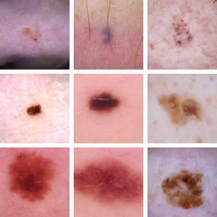
We evaluate the hierarchical pyramid CAN on two medical classification benchmarks. CAN-1 CAN-2 and CAN-3 denote three compact pyramid variants with different capacity budgets. Both datasets are resized to 224×224 before being input to the network.
| Kvasir-Dataset-v2 | ISIC2018 |
|---|---|
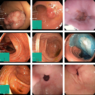 |  |
Kvasir-Dataset-v2
| resnet50 | densenet161 | vit-small | convnext_tiny | efficientvit | CAN-1 | CAN-2 | |
|---|---|---|---|---|---|---|---|
| Acc | 88.50% | 89.08% | 75.50% | 77.83% | 82.83% | 91.58% | 90.33% |
| MCC | 0.8689 | 0.8756 | 0.7209 | 0.7471 | 0.8041 | 0.9039 | 0.8902 |
| Params | 23.5M | 26.5M | 21.7M | 27.8M | 6.58M | 1.66M | 0.36M |
ISIC2018
| resnet50 | densenet161 | vit-small | convnext_tiny | efficientvit | CAN-3 | CAN-2 | |
|---|---|---|---|---|---|---|---|
| Acc | 80.15% | 82.88% | 67.13% | 78.95% | 80.45% | 86.43% | 86.23% |
| MCC | 0.6056 | 0.6658 | 0.4109 | 0.5824 | 0.6050 | 0.7398 | 0.7326 |
| Params | 23.5M | 26.5M | 21.7M | 27.8M | 6.58M | 0.89M | 0.36M |
Observation: The pyramid CAN consistently improves the accuracy/efficiency trade-off on both datasets.
CAN-1gives the strongest top-line accuracy, whileCAN-2retains competitive performance with only 0.36M parameters. For all models on the medical datasets, we train from scratch for 200 epochs.
🛠️ Usage
CliffordNet supports two execution modes: a High-Performance Mode (using custom CUDA kernels) and a Compatibility Mode (pure PyTorch).
Requirements:
torch>=2.0.0
python>=3.10
1. Installation (Hardware Acceleration)
Install the compiled clifford_thrust wheel matching your environment。
⚠️ Note: The provided wheels are currently optimized and tested specifically for NVIDIA RTX 4090 (Compute Capability 8.9). For other GPUs, please use the standard PyTorch mode.
-
Python 3.10 + CUDA 11.8
pip install cuda/clifford_thrust-0.0.1-cp310-cp310-linux_x86_64.whl -
Python 3.12 + CUDA 12.8
pip install cuda/clifford_thrust-0.0.1-cp312-cp312-linux_x86_64.whl
2. Training
To launch training, simply run the script. The code automatically handles the fallback if the accelerated kernels are not installed.
-
Accelerated Mode (Recommended): Requires
clifford_thrustinstalled.python train.py --enable_cuda -
Standard Mode (Pure PyTorch): Works on any device (MPS/CUDA) without extra dependencies.
python train.py
3. Python API & Model Zoo
You can instantiate the models directly using the CliffordNet class. Below are the configurations for our top-performing variants.
from model import CliffordNet

# ---------------------------------------------------------
# 1. CliffordNet-Nano (1.4M)
# ---------------------------------------------------------
model_nano = CliffordNet(
    num_classes=100,
    patch_size=2,
    embed_dim=128,
    depth=12,
    cli_mode='full',
    ctx_mode='diff',
    shifts=[1, 2],
    drop_path_rate=0.3
)

# ---------------------------------------------------------
# 2. CliffordNet-Lite (2.6M)
# ---------------------------------------------------------
model_lite = CliffordNet(
    num_classes=100,
    patch_size=2,
    embed_dim=128,
    depth=12,
    cli_mode='full',
    ctx_mode='diff',
    shifts=[1, 2, 4, 8, 16],
    drop_path_rate=0.3
)
For pyramid experiments, instantiate the hierarchical backbone directly:
from model_hier import HierarchicalCliffordNet

model = HierarchicalCliffordNet(
    num_classes=8,
    patch_size=2,
    cli_mode="full",
    ctx_mode="diff",
    shifts=(1,),
    stage_depths=(3,4,5),
    stage_dims=(32,64,96),
    downsample_mode="conv",
    drop_path_rate=0.1,
    enable_cuda=True,
)
The same interface can be scaled by modifying:
stage_depths: number of Clifford blocks in each stage.stage_dims: channel width of each pyramid level.shifts: channel-wise Clifford interaction offsets.downsample_mode: one ofavgpool,conv, orpatch.
🖊️ Citation
If you find this work helpful, please cite us:
@article{2026cliffordnet,
  title={CliffordNet: All You Need is Geometric Algebra},
  author={Zhongping Ji},
  journal={arXiv preprint arXiv:2601.06793},
  year={2026}
}
🙏 Acknowledgement
We thank the open-source community for the implementations of timm, which facilitated our baseline comparisons.